


Next: Program structure
Up: paper
Previous: Introduction
This generator simulates
the  interaction:
 where
where
 and
and  indicate the
electron/positron and the proton in the initial state respectively,
indicate the
electron/positron and the proton in the initial state respectively,
 and
and  are
the scattered electron/positron and the produced dilepton respectively.
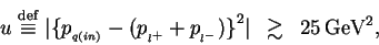
The relevant processes are classified into 3 categories using
the negative momentum transfer squared at the proton vertex(
are
the scattered electron/positron and the produced dilepton respectively.
The relevant processes are classified into 3 categories using
the negative momentum transfer squared at the proton vertex( ) and
the invariant mass of the hadronic system(
) and
the invariant mass of the hadronic system( );
);
 |
(1) |
 |
(2) |
where
 and
and  are the 4-momenta of
the incoming lepton and the proton after ISR, respectively.
are the 4-momenta of
the incoming lepton and the proton after ISR, respectively.
 and
and
 are those of the scattered
lepton and the produced leptons before FSR, respectively.
The 3 categories are
are those of the scattered
lepton and the produced leptons before FSR, respectively.
The 3 categories are
 ( elastic),
-
 OR
OR
 ( quasi-elastic),
-
 AND
AND
 ( DIS),
where  and
and  are the masses of the proton and the neutral pion,
respectively.
are the masses of the proton and the neutral pion,
respectively.
 is set to around 1GeV depending on the Parton Density Function (PDF)
used in the DIS process.
The recommended value for
is set to around 1GeV depending on the Parton Density Function (PDF)
used in the DIS process.
The recommended value for  is 5GeV.
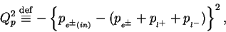
For the elastic process, the diagrams in Fig.1
are calculated with the following dipole form factor
for the proton-proton-photon vertex
(
 ) with the on-shell proton.
The general form of the elastic proton vertex can be written as
) with the on-shell proton.
The general form of the elastic proton vertex can be written as
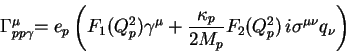 |
(3) |
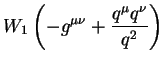
where  indicates the electric charge of the proton,
 is the 4-momentum transfer at the proton vertex (
 ),
),
 and
and  are the 2 independent form factors,
and
are the 2 independent form factors,
and  is the anomalous magnetic moment of the proton
(see, for example, [#!Q_and_L!#].).
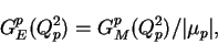
The electric and magnetic form factors
is the anomalous magnetic moment of the proton
(see, for example, [#!Q_and_L!#].).
The electric and magnetic form factors
 and
and
 , respectively
are defined as follows,
, respectively
are defined as follows,
 |
(4) |
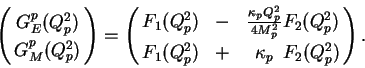
Using the Gordon decomposition and the scaling law of the form factor,
 |
(5) |
the following formula which is used in this program is obtained,
 |
(6) |
where
 ,
,  is the Bohr magneton,
and
is the Bohr magneton,
and  indicates the 4-momentum of the scattered proton.
is calculated according to the formula of the dipole fit,
indicates the 4-momentum of the scattered proton.
is calculated according to the formula of the dipole fit,
 |
(7) |
The only difference between the elastic and the quasi-elastic processes is
the treatment of the proton vertex and
the simulation of the hadronic final state.
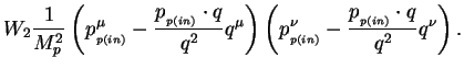
The quasi-elastic proton vertex can be described using the hadron tensor
in the following form assuming parity and
current conservation (for example, see [#!Q_and_L!#].),
 and
and
 are
the electromagnetic proton structure functions.
The hadron tensor is contracted with
the lepton tensor
are
the electromagnetic proton structure functions.
The hadron tensor is contracted with
the lepton tensor  numerically to obtain the cross section,
 |
(9) |
In this version,
 and
and  are parameterized with Brasse et al.[#!BRASSE!#]
for
are parameterized with Brasse et al.[#!BRASSE!#]
for  2GeV (the proton resonance region),
and with ALLM97 [#!ALLM97!#] for
2GeV (the proton resonance region),
and with ALLM97 [#!ALLM97!#] for  2GeV.
These two parameterizations are based on fits to the experimental data
on the measurement of the total
2GeV.
These two parameterizations are based on fits to the experimental data
on the measurement of the total  cross-sections.
The exclusive hadronic final state is generated
using the MC event generator SOPHIA [#!SOPHIA!#]
in the event generation step.
cross-sections.
The exclusive hadronic final state is generated
using the MC event generator SOPHIA [#!SOPHIA!#]
in the event generation step.
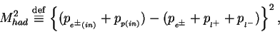
For the DIS process with the Quark Parton Model,
the diagrams in Fig.2 are calculated.
PDFLIB [#!PDFLIB!#] is linked to obtain parton densities
with as a QCD scale.
The simulation of the proton remnant and the hadronization are
performed by PYTHIA [#!PYTHIA!#].
It should be noted that the lowest order calculation in this process is valid only
for the region of
 |
(10) |
where  is the 4-momentum of the incoming quark.
The value of
is the 4-momentum of the incoming quark.
The value of  corresponds to the virtuality of the -channel quark
in the diagrams in Fig.2-(b),(c).
When it is nearly or smaller than 25 GeV
corresponds to the virtuality of the -channel quark
in the diagrams in Fig.2-(b),(c).
When it is nearly or smaller than 25 GeV ,
the lowest order calculation is not correct as explained in [#!EPVEC!#]
since QCD corrections become large.
In this case, the dilepton production should be treated as Drell-Yan process
between the proton and the resolved photon from the beam lepton,
which is not implemented in this program.
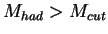
The cut:
,
the lowest order calculation is not correct as explained in [#!EPVEC!#]
since QCD corrections become large.
In this case, the dilepton production should be treated as Drell-Yan process
between the proton and the resolved photon from the beam lepton,
which is not implemented in this program.
The cut:  GeV is explicitly applied in this program
if the diagrams other than BH are included.
GeV is explicitly applied in this program
if the diagrams other than BH are included.
The effect of ISR is included in the cross-section calculation using
the structure function method described in [#!ISR_SF!#],
where the momentum transfer squared on the beam lepton,
i.e.
 is used as a QED scale.
When ISR turns on, the correction for the photon self energy,
i.e. the vacuum polarization,
is included according to the parameterization in [#!QEDVAC!#]
by modifying photon propagators.
FSR is performed by PYTHIA using the parton shower method
when the event is generated.
is used as a QED scale.
When ISR turns on, the correction for the photon self energy,
i.e. the vacuum polarization,
is included according to the parameterization in [#!QEDVAC!#]
by modifying photon propagators.
FSR is performed by PYTHIA using the parton shower method
when the event is generated.
Fig. 1:
Feynman diagrams included in the (quasi-)elastic process.
 =
=
 ,
l
,
l =
=
 .
N means a (dissociated) proton or a nucleon resonance.
.
N means a (dissociated) proton or a nucleon resonance.
|
|
Fig. 2:
Feynman diagrams included in the DIS process.
=
,
l=
and
=


 ,
,


 ,
, ,
, ,
, ,
,
 .
.
|
|
Next: Program structure
Up: paper
Previous: Introduction
Tetsuo Abe
2001-07-12
![\includegraphics[scale=1.0,clip]{pictures/diagrams_GRAPE_ela}](img76.gif)
![\includegraphics[scale=0.8,clip]{pictures/diagrams_GRAPE_dis}](img80.gif)