CAVITY MODIFICATIONS AND LOW POWER TESTS OF THE KEK RFQ/IH LINAC

JAERI and KEK are constructing jointly Tokai Radioactive Ion Accelerator Complex (TRIAC) facility since fiscal year 2001 at JAERI-Tokai tandem site [1]. In the first stage, radioactive ion beams from the ISOL are accelerated by a split coaxial RFQ (SCRFQ) and an interdigital-H (IH) linac up to the energies of 0.14 to 1.09 MeV/u. In the second stage, the beam from the SCRFQ and IH linac is accelerated by an IH2 linac up to 2-MeV/u, and further accelerated by the superconducting (SC) linac up to the energy above Coulomb barrier. The maximum beam energies are 5 MeV/u for q/A=1/7 ions and 8 MeV/u for q/A=1/4 ions.
We modified the existing SCRFQ and IH cavities to match their resonant frequencies to that of the SC linac. Since the resonant frequency of SC linac is 129.8 MHz, the frequency of SCRFQ has been changed from 25.5 to 25.96 MHz and that of IH from 51 to 51.92 MHz.

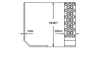
Figure 1:Shape of the C-tuner.	SCRFQ Resonant frequency and inter-vane voltage along beam axis were well tuned by changing locally inter-vane capacitance and stem (used for supporting the vanes) inductance. For changing the capacitance, C-tuners of the copper plates (Fig. 1) were attached on the back-plates of the vanes so that a plate confronted a stem with a distance of 25 mm. We adjusted the stem inductance by changing the area of the stem-flange windows with panels (Fig. 2). For tuning the frequency and field distribution, height of the C-tuners installed in the first, second and 12th modules was changed as shown in Table 1; the number of tuners is four per module. Height of the panels before and after tuning is summarized in Table 2.
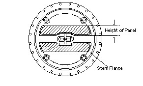
Figure 2:Panels attached on the stem flange.	Table1: Height of C-tuners installed in the first, second and 12th modules 1st module 2nd module 12th module Height of C-tuners before tuning (mm) 170 120 120 Height of C-tuners after tuning (mm) 170 70 95
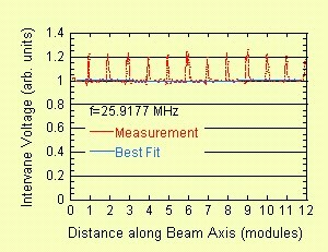
Figure 3:Longitudinal inter-vane voltage distribution.	Table2: Height of Panels attached on the stem flanges before tuning after tuning Positions of the stem flanges Height of panels Positions of the stem flanges Height of panels Between 3rd and 4th modules 0mm Between 3rd and 4th modules 136.5mm Between 6th and 7th modules 125mm Between 6th and 7th modules 136.5mm Between 9th and 10th modules 0mm Between 9th and 10th modules 136.5mm Values of the capacitance and inductance to be changed were estimated by using an equivalent circuit analysis [2]. For the inter-vane voltage measurements, a Teflon perturbing object of a square plate, 30×30×8mm3, was moved along two vanes used as a guide. Figure 3 shows the measured longitudinal inter-vane voltage distribution of the SCRFQ.
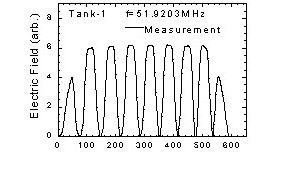
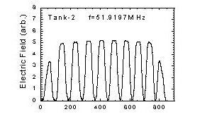
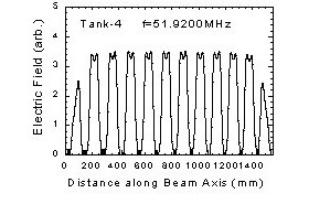
Figure 4:Electric field distributions.	IH linac The resonant frequencies were tuned by increasing the gap lengths between drift-tubes, that is, by decreasing the capacitance. For increasing the gap length, the drift-tube length was shortened. All drift-tubes except end drift-tubes were replaced to the modified ones. Dimensions of the drift-tubes were finally determined by model tests after rough estimations by MAFIA calculations [3]. Each cavity of IH Linac has a capacitive tuner and a inductive one. They change the frequency 100 or 150 kHz. Therefore, we tuned the frequency to the goal one with an accuracy better than ±50kHz . For the field measurements, a perturbing bead was moved along the beam axis. The bead is an aluminum sphere of 6.3 mm in diameter. Figure 4 shows the measured electric field distributions along beam axes of the IH cavities.

References
[1] S. Arai et al., Proc. of EPAC 2002, Paris, France, 2002, p.861.
[2] S. Arai, KEK Report 2001-7, 2001.
[3] Y. Arakaki et al., Proc. of EPAC 2002, Paris, France, 2002, p.864.